Global Navigation Satellite System (GNSS) receivers convert weak radio signals from satellites into precise positioning and timing information. This involves several signal processing stages: signal acquisition, signal tracking, decoding navigation data, and computing position solutions. In this section, we focus on GNSS receiver design and signal processing techniques, covering receiver architecture and key algorithms for acquisition, correlation, tracking, and mitigation of errors. (We avoid overlapping with fundamental GNSS concepts or positioning solution techniques, and concentrate on the receiver’s internal processing.)
Receiver Architecture
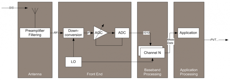
Figure 1: A generic GNSS receiver architecture. The antenna feeds an RF front-end that down-converts, amplifies, and digitizes the satellite signals (producing in-phase I and quadrature Q samples). Dedicated digital signal processing channels then acquire and track each satellite’s signal in parallel, and a navigation processor computes the Position/Velocity/Time (PVT) solution (Meas. Data = measurements output)[1][2].
A typical GNSS receiver consists of several building blocks[1]:
- Antenna: Usually a Right-Hand Circularly Polarized (RHCP) antenna tuned to the GNSS L-band frequencies (
1–2 GHz). It captures the direct satellite signals (Signals In Space, SIS) while minimizing multipath and interference. Many GNSS antennas include a low-noise preamplifier and filtering stage to boost the very weak signals (–130 dBm) and reject out-of-band noise[3][4]. High-precision antennas (e.g., choke-ring designs or multi-element arrays) further reduce multipath by shaping the reception pattern (strong gain at high elevations, attenuation toward the horizon)[5][6]. - RF Front-End: This analog front-end down-converts and digitizes the incoming RF signals[7]. In a traditional superheterodyne architecture, the front-end uses a local oscillator (LO) to mix the L-band signal down to an intermediate frequency (IF in the MHz range), then band-pass filters and amplifies it (often with automatic gain control, AGC), and finally an analog-to-digital converter (ADC) samples the signal into I/Q baseband components[8]. The front-end design must ensure sufficient bandwidth for the GNSS signals (e.g., ~2 MHz for GPS L1 C/A, up to ~20–24 MHz for modern wideband signals like Galileo E5), and use a low-phase-noise oscillator for frequency stability[9]. Some modern receivers employ direct-conversion or direct sampling architectures, where the RF or IF signal is sampled directly by a high-speed ADC, eliminating some analog stages at the cost of increased ADC performance requirements. Key front-end parameters include the LO stability (e.g., temperature-compensated crystal oscillators are common, whereas high-end receivers may use even more stable oscillators for better phase stability[9]) and the frequency plan (choosing IF and sampling rates to avoid interferences, images, or aliasing). The output of the front-end is a digitized baseband (or low-IF) stream containing the spread-spectrum signals of all visible satellites.
- Baseband Signal Processing (Channels): The digital baseband section contains multiple parallel channels (tracking channels), each devoted to acquiring and tracking one GNSS satellite signal[2][10]. Each channel generates a replica of a specific satellite’s code and carrier, then mixes (correlates) it with the incoming I/Q samples to acquire the signal and maintain lock with it (signal tracking). Each channel typically implements at least a code Delay-Lock Loop (DLL) to track the code phase (for pseudorange measurement) and a carrier Phase-Lock Loop (PLL) to track the carrier frequency/phase (for Doppler and phase measurements)[2]. The baseband processor usually also includes integration and filtering blocks, discriminators for the loops, and sometimes additional aiding logic (for example, aiding the DLL with the PLL output, or adapting loop bandwidths based on signal conditions[11]). The number of channels dictates how many satellites and frequencies can be tracked in parallel (e.g., a “12-channel receiver” can track 12 signals, which could be 12 satellites on one frequency, or fewer satellites on multiple frequencies depending on configuration).
- Navigation/Applications Processor: Finally, the receiver’s navigation processor uses the measured pseudoranges, carrier phases, Doppler frequencies, and decoded satellite messages from all tracked channels to compute the user’s position, velocity, and time solution (the PVT)[12]. It also handles decoding of the navigation data (ephemerides, clock corrections, etc.), and may apply error corrections or sensor fusion as needed. In high-end or application-specific receivers, this stage may output additional information such as signal quality metrics (e.g., carrier-to-noise density $C/N_0$ for each signal)[13], atmospheric data, or act as part of a larger integrated system. Practical design considerations at this stage include what outputs are needed (e.g., raw measurements for post-processing vs. only PVT), update rate, and interfacing with external systems or protocols.
Design Trade-offs: Receiver architectures are influenced by the target application and required performance[14]. For example, a low-cost mass-market receiver (like those in smartphones) is typically single-frequency (L1-only), highly integrated with other radio functions, and optimized for low power consumption and size. In contrast, a geodetic-grade or reference receiver may be multi-frequency (tracking GPS L1/L2/L5, Galileo E1/E5, etc.), with very low-noise clocks and antenna arrays, to achieve maximum accuracy and reliability. Multi-constellation support (GPS, GLONASS, Galileo, BeiDou, etc.) greatly improves satellite availability and robustness in challenging environments, but requires more channels and more complex RF front-ends (e.g., GLONASS uses frequency-division multiple access, so the front-end or digital processing must accommodate different frequencies for each satellite)[14]. Designers must balance factors such as sensitivity, accuracy, update rate, power consumption, and cost. As an example, increasing front-end bandwidth can improve multipath resolution and tracking performance, but will also amplify noise and demands on the ADC; using narrower correlator spacing in the DLL can reduce multipath error (as discussed later) at the cost of more complex tracking loops. Table 1 summarizes a few architecture variants and their typical usage:
| Architecture Type | Description and Use Case | Pros | Cons |
|---|---|---|---|
| Conventional HW Receiver | Dedicated hardware (ASIC/FPGA) for GNSS baseband. Common in mass-market devices (phones, car nav) and some professional receivers. | Low power and real-time operation; optimized tracking loops in silicon. | Less flexible – hard to support new signals or algorithms once built. |
| Multi-Frequency Survey Receiver | High-end receiver with multiple RF front-ends or wide-band front-end to track several frequencies (e.g., L1+L2+L5 for GPS, and corresponding bands for other constellations). Often uses high-stability oscillator (OCXO or atomic). | Very high accuracy (cm-level with RTK) and robust multipath mitigation; can correct ionospheric delay by combining frequencies. | High cost and power; larger size; needs good antenna (often choke-ring or multi-element). |
| Direct RF Sampling Receiver | Architecture where the GNSS signal is directly digitized at RF or with minimal analog processing. Uses a high-speed ADC and DSP. Seen in some modern receivers and research prototypes. | Simplified analog design (no multiple mixing stages); very flexible in digital domain (can tune to any frequency band via software). | Requires extremely fast ADC and processor -> higher power usage; ADC dynamic range and noise are critical. |
| Vector Tracking Receiver | An advanced design where tracking loops for all satellites are coupled via a common navigation filter (EKF or Kalman filter) rather than independent scalar loops. Mainly in research and specialized applications (e.g., high dynamics). | Better handling of signal outages or dynamics by sharing info across channels; can improve sensitivity and robustness. | Computationally complex; can be less stable if not tuned well; not widely used in commercial receivers yet. |
| High-Sensitivity Receiver | A receiver optimized for very weak signals (e.g., indoors). Uses long integration times, aiding data, and perhaps massive parallel correlation. Often integrated in assisted-GPS (A-GPS) systems in phones. | Can acquire signals down to very low C/N₀ by coherent integration over many milliseconds and using aiding (time, position, satellite data). | Long time to get fixes without assistance; reduced accuracy of timing; specialized use (when signals are extremely weak). |
| Software-Defined Receiver (SDR) | Implements RF signal processing in software on a general-purpose processor or FPGA, using a generic RF front-end. Often used in research, prototyping, and special applications (described in detail later). | Unparalleled flexibility (new signals or algorithms via software updates; can log and re-process raw data offline; easy to integrate other sensors). | Much higher processing power needed (often orders of magnitude more power consumption than ASIC); not power-efficient for handheld use; depends on high-throughput data transfer from RF front-end.[15] |
This list is not exhaustive, but illustrates how receiver design choices align with different goals. In practice, many GNSS receivers combine approaches – for example, a modern automotive receiver might use a multi-constellation hardware ASIC for core tracking, but also output raw measurements for sensor fusion (an element of SDR flexibility). Regardless of architecture, all GNSS receivers must perform two fundamental processing steps: acquisition of the satellite signals, and tracking of those signals to extract measurements. We turn to those next.
Signal Acquisition and Tracking (DLLs, PLLs)
Signal Acquisition is the initial process of detecting a satellite’s signal and coarse alignment of its code and frequency. When a receiver is first powered on (or when tracking of a satellite is lost), it must search for which satellites are visible and find their signal parameters. The receiver knows each satellite’s unique PRN code sequence (via GNSS specifications), but it does not initially know the code’s time offset or the Doppler shift of the signal[16][17]. Acquisition involves a search over a two-dimensional space: code phase (ranging from 0 to the full code length) and Doppler frequency (within ±5–10 kHz or more, depending on receiver motion and satellite velocity)[18][19]. In other words, the receiver tries different time alignments of a replica PRN code against the incoming signal, and for each alignment it tries different frequency offsets to account for Doppler. When the correct code delay and frequency are tried together, the correlator output shows a strong correlation peak, indicating the signal is found[19].
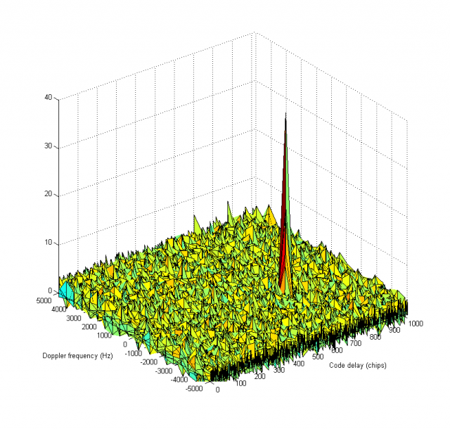
Figure 2: Example acquisition correlation search space across code phase (chips) and Doppler frequency (Hz). The 3D plot shows the correlation power resulting from trying various code delays (x-axis) and frequency offsets (y-axis). A strong correlation peak (red spike) appears when the locally generated code and carrier frequency match the incoming satellite signal, here at approximately 650 chips delay and –1750 Hz Doppler[19]. In practice, the receiver identifies this peak as a detected satellite.
In a basic acquisition strategy, the receiver performs a brute-force search: it slides the replica code in time (typically in steps of 0.5 or 1 chip) and steps through a range of Doppler offsets (perhaps every 500 Hz)[20][21]. The search space can be large; for example, acquiring a GPS L1 C/A signal might involve up to 1023 possible code phases × ~41 frequency bins (for ±10 kHz at 500 Hz steps) for each of 32 satellites[22]. This naive search would require correlating many thousands of combinations, which is computationally intensive. To accelerate acquisition, parallel search techniques are used: modern receivers often perform part of the search in the frequency domain using FFT-based methods (circular correlation), enabling many code offsets to be tested at once. Some architectures use dedicated hardware correlator banks to test multiple Doppler bins in parallel. Additionally, assistance data (as in Assisted-GPS) can drastically reduce the search space: approximate time and position allow the receiver to predict which satellites should be visible and their Doppler shifts, so it only searches around those predictions[23]. Using such aiding (e.g., from a network almanac or prior fix) the acquisition can be much faster, because the satellite dimension and much of the frequency uncertainty are narrowed down[24].
Acquisition is typically declared successful if the correlation peak exceeds a certain threshold above the noise floor, indicating a lock. Once a satellite is acquired (i.e. rough code phase and Doppler are known), the receiver enters the tracking stage for that signal.
Signal Tracking is the continuous process of fine-tuning the alignment of the local signal replica (code phase and carrier frequency/phase) to remain locked onto the satellite’s signal. Tracking is achieved using feedback loops that adjust the replica in real-time, as the satellite-receiver geometry changes (causing Doppler and code phase shifts)[25][26]. The principal tracking loops in a GNSS receiver are:
- Delay-Locked Loop (DLL): A feedback loop that tracks the code phase (timing) of the PRN code. It keeps the receiver’s locally generated code in sync with the incoming satellite code by measuring early vs. late timing errors.
- Phase-Locked Loop (PLL): A loop that tracks the carrier phase of the incoming signal. It corrects differences between the incoming carrier wave’s phase and a locally generated carrier (NCO) to maintain phase alignment.
- Frequency-Locked Loop (FLL): Sometimes used (especially during acquisition or for highly dynamic situations) to track the carrier frequency (Doppler) when phase lock is not yet achieved. An FLL can coarsely track large frequency changes and hand off to a PLL for fine tracking.
All these loops are classic negative feedback control systems[27][28]. They work by producing an error signal (via a discriminator) that indicates how far off the replica is from the incoming signal, then filtering that error and feeding it back to adjust the local code generator or oscillator in the opposite direction (negative feedback) to reduce the error. For example, if the code replica is lagging behind the incoming signal, the DLL’s discriminator output will indicate a positive error, and the loop will slightly increase the code NCO frequency to catch up until the error is zero.
In practice, a GNSS receiver’s tracking stage employs a carrier PLL (often aided by an FLL) to handle the carrier Doppler and phase, and a code DLL to handle the code delay. These loops operate in tandem on each channel. Initially, right after acquisition, the frequency uncertainty is still large, so a wider-bandwidth FLL-assisted-PLL might be used: the FLL quickly locks the frequency within a few tens of Hz, then the receiver switches to a PLL for precise phase tracking[29][30]. Meanwhile, the DLL starts tracking the code with the aid of the carrier lock (since carrier phase can provide a much finer measurement of range change, the receiver often uses the Doppler/PLL output to help the code tracking). Once in steady-state tracking, the DLL and PLL keep the local replica aligned by adjusting for changes in range (code phase) and range rate (Doppler).
The design of tracking loops involves selecting loop parameters such as loop bandwidth and integration time. A narrow bandwidth (e.g., a PLL bandwidth of say 5 Hz versus 15 Hz) means the loop is more selective and smooths out more noise, yielding less phase jitter, but it responds more slowly to dynamics (e.g., rapid acceleration of the receiver)[31][32]. Longer integration times (coherent or non-coherent integration over multiple milliseconds) improve sensitivity by averaging out noise, but can be limited by dynamics or data bit transitions on the signal[33]. Receivers often adapt loop settings based on conditions: for instance, when signal $C/N_0$ is high and dynamics are low, very narrow loops can be used for maximum precision; in high dynamics or low $C/N_0$ situations, loop bandwidths may be widened to avoid loss of lock[11]. Modern receivers may implement adaptive loop bandwidth control algorithms that adjust these parameters on the fly[11].
Each tracking channel continuously produces measurements: pseudorange (from the DLL, based on code phase offset), Doppler frequency (from the frequency/phase loop, related to range rate), and carrier phase (accumulated phase from the PLL, for high-precision positioning), as well as decoded bits of the navigation message. To maintain lock, the receiver must also handle challenges such as signal fading or data bit flips. Next, we examine in more detail the correlation process and code tracking, followed by the carrier phase tracking aspects.
Correlation and Code Tracking
Correlation is the fundamental operation in GNSS signal processing that allows the receiver to “match” the incoming signal to a known PRN code. Correlation can be thought of as a sliding dot-product: the receiver multiplies the incoming signal by a locally generated PRN code sequence and accumulates (integrates) the result over a short period (the integration time). When the locally generated code aligns with the satellite’s code in the incoming signal (and the correct Doppler shift is removed), the correlator output is maximized (the correlation peak)[34][35]. Mathematically, an ideal correlation (over a time $T$) can be expressed as an integral (or sum for digital samples):
where $s_{\text{recv}}(t)$ is the received signal (at IF or baseband) and $c_{\text{loc}}(t)$ is the locally generated PRN code (with a time offset $\tau$). The correlation $R(\tau)$ as a function of the code offset $\tau$ will show a sharp peak when $\tau$ equals the actual code delay of the satellite signal. In practice, the incoming signal is noisy and also modulated by a carrier, so the receiver mixes the signal to baseband (removing Doppler) and performs discrete-time correlations for several trial $\tau$ values until the peak is found (acquisition)[18]. During tracking, correlation is performed continuously at the expected $\tau$ (and perhaps a few offsets around it to measure the error).
Because GNSS signals are Direct Sequence Spread Spectrum, the correlation function has a shape determined by the PRN code autocorrelation. For example, the GPS L1 C/A code autocorrelation has a triangular main lobe about 1 chip wide (1 µs or ~300 m in code delay) and near-zero values elsewhere (aside from some sidelobes). Modern binary offset carrier (BOC) modulations, used in Galileo and modernized GPS signals, produce autocorrelation functions with multiple peaks (a narrower main peak but with side-peaks due to the sub-carrier modulation)[36]. The receiver’s tracking loops must ensure they lock onto the correct main peak and not a side-peak. Techniques for unambiguous tracking of BOC signals include narrowing the tracking range or using additional correlators to detect side-peak lock. One example is the “bump-jumping” algorithm, which adds extra “very early” and “very late” correlators to monitor the correlation at offsets corresponding to potential side peaks; if the side correlations become larger, the loop can “jump” to the correct peak[36]. This ensures the DLL stays on the true correlation peak of a BOC signal rather than a false lock.
In a standard receiver’s Delay-Lock Loop (DLL) for code tracking, the typical implementation uses multiple correlators: one aligned slightly Early of the prompt signal, one Prompt, and one Late by a small offset (δ) in code phase (e.g., ±0.5 chip around the prompt). The DLL computes an error signal based on the difference between the Early and Late correlator outputs, which indicates if the replica code is leading or lagging the incoming code[37][38]. A common discriminator formula for a non-coherent DLL is:
where $(I_E, Q_E)$ and $(I_L, Q_L)$ are the I/Q correlator values for the Early and Late replicas respectively. When the prompt is exactly aligned with the signal, the Early and Late correlations are equal, yielding zero error. If Early correlator is stronger, the replica is too early and must be delayed, and vice versa[39]. The loop filter then adjusts the code NCO (Numerically Controlled Oscillator) to drive this error to zero, keeping the code lock. Traditionally, GPS receivers used an Early-Late spacing of one full chip (1.0 chip) for the C/A code, but this was found to be suboptimal in presence of multipath. A narrow correlator technique reduces the Early-Late spacing (e.g., to 0.1 chip or even less) to narrow the spacing of the correlation power around the peak[40]. By using a smaller correlator spacing, the DLL becomes much less sensitive to delayed multipath signals, effectively sharpening the timing discrimination. In fact, a receiver using a 0.1-chip narrow correlator and a wider pre-correlation bandwidth can achieve code tracking accuracy nearly as good as a P(Y)-code receiver on L1 (which inherently has a much higher chipping rate)[41]. This innovation, first described by Van Dierendonck and others in the early 1990s, dramatically reduced multipath-induced range errors for C/A code users[41]. Strobe correlators (or double-delta correlators) extended this idea by using multiple narrow correlators with certain weighting patterns to further flatten the error curve in presence of short-delay multipath[42].
The correlator architecture can go beyond the basic Early-Prompt-Late trio. Multi-correlator designs use many correlators per channel to gather more information about the correlation function shape. For example, the Multipath Estimating DLL (MEDLL) uses perhaps 5 or 10 correlators spanning the main lobe of the autocorrelation function[43]. By fitting a model of multiple signal paths to these correlator outputs (using maximum-likelihood estimation), MEDLL explicitly estimates the delays and amplitudes of individual multipath signals. It then subtracts the contribution of secondary multipath components from the correlation, leaving an estimate of the direct signal correlation peak, which yields a more accurate pseudorange[43]. This method requires more computation, but it can significantly improve code tracking accuracy in multipath environments. Other advanced techniques like Multipath Mitigation Technology (MMT) and the Vision Correlator have been developed to improve on these concepts[42]. In summary, the design of the code tracking loops and correlator spacing is crucial for mitigating errors – narrow correlators and advanced multi-correlator techniques help attain more robust tracking especially when facing multipath.
Another aspect of code tracking is that modern GNSS signals often have a data channel and a pilot channel (e.g., Galileo E1B (data) and E1C (pilot), or GPS L2C/L5 which have a pilot component without data). A pilot channel has no navigation data bit flips, which allows the receiver to integrate the signal for longer periods and track the phase without 180° ambiguities. When a pilot is available, the receiver’s PLL/DLL can operate on that signal for improved stability, and use the data channel primarily for reading the nav message. For signals that do include data (e.g., GPS L1 C/A with 50 Hz bit rate), the code tracking loop usually isn’t affected by the bit flips (since the code correlation can span many bits), but the carrier tracking needs special handling (see next section on carrier tracking).
In summary, the correlation and code tracking stage provides a continuous lock on the satellite’s code timing, yielding the fundamental measurement of pseudorange (travel time of the signal). It does so by utilizing one or more correlators and a DLL feedback loop, with design choices like correlator spacing and integration time impacting the performance (noise vs. multipath trade-offs). Next, we discuss carrier phase tracking, which provides even more precise measurements by tracking the signal’s carrier wave.
Carrier Phase Tracking
While the code tracking loop provides pseudorange with an accuracy on the order of a meter (limited by the code chip length and noise), carrier phase tracking enables measurements with millimeter-level precision. The carrier phase of a GNSS signal (at L1 frequency ~1575.42 MHz, wavelength ~19 cm, or other bands with similar cm-level wavelengths) can be tracked to a fraction of a cycle. By counting the cycles of the carrier signal from transmission to reception (and accounting for the integer number of cycles ambiguities), the receiver can obtain a relative range measurement with an extremely fine resolution (on the order of 0.01 m or better). This is the basis for high-precision techniques like Real-Time Kinematic (RTK) and Precise Point Positioning (PPP)[44].
The Phase-Locked Loop (PLL) in a GNSS receiver is responsible for tracking this carrier phase. In a PLL, the receiver generates a replica carrier (using a numerically controlled oscillator, NCO) and adjusts its phase and frequency to match the incoming signal’s carrier. The discriminator in a PLL measures the phase error – basically how much the prompt correlator’s output is off from entirely in-phase. Ideally, when perfectly locked, all the signal power comes into the In-Phase (I) correlator and the Quadrature (Q) correlator output is zero (for a data-less signal)[45][46]. Any phase misalignment will cause some energy to appear in Q, which the discriminator detects. A simple phase discriminator is $ \theta_{\text{err}} = \arctan2(Q_P,,I_P)$, the four-quadrant arctangent of the prompt I and Q values[47]. This gives the phase error directly, but has a complication: if the signal has data bits (which can cause 180° phase reversals), the arctan would jump when a bit flips (because the sign of $I_P$ and $Q_P$ flips). Therefore, receivers typically either wipe off the data bits (if they know them from decoding or if working on a pilot channel), or use a Costas loop discriminator which is insensitive to data bit flips[48]. The Costas loop effectively tracks the carrier power regardless of bit sign by using a two-quadrant discriminator. For example, a classical Costas discriminator multiplies $I_P$ and $Q_P$ (or uses $\operatorname{atan2}(Q, |I|)$) to get an error signal that depends on $2\phi_e$ but not on the sign of $I_P$[48]. In practice, one common implementation is:
which is approximately $\sin(2\phi_e)$ for small phase errors[48]. When the incoming signal flips phase (due to a data bit), both $I_P$ and $Q_P$ flip sign, and their product $I_P Q_P$ does not change sign, thus the Costas loop “sees” no phase jump. This allows continuous tracking through navigation data bit transitions.
The PLL typically has a higher bandwidth than the DLL (because carrier phase can change rapidly with dynamics, and also to quickly respond to any data-bit-induced errors if not fully wiped off). However, it is also more sensitive to noise – at low $C/N_0$, the PLL is usually the first to lose lock. The thermal noise-induced phase jitter in a PLL can be approximated by formulae from control theory[49][50], which show it increasing with loop bandwidth $B_n$ and decreasing with higher $C/N_0$ and longer integration $T$. As mentioned, choosing a loop bandwidth is a trade-off: a narrow PLL (say 1–2 Hz) yields very low phase noise (good for precision) but cannot follow rapid phase changes (bad for high dynamics or oscillator drift), whereas a wide PLL (say 15 Hz) can track faster changes but at the cost of more noise in the phase observable[31]. Some receivers implement an Adaptive PLL that starts wide to lock quickly and under dynamic conditions, then narrows when the signal is stable to improve precision[11].
Carrier phase measurements are ambiguous by an integer number of wavelengths – the receiver can only measure the fractional phase (0 to 1 cycle) unambiguously, while the total range could have an unknown integer number of full cycles (each ~19 cm for L1) between satellite and receiver. These integer ambiguities are resolved in techniques like RTK by having a reference receiver and user receiver observe the same satellites and then using algorithms (often based on differencing measurements and searching for integer solutions) to fix the cycle ambiguities. Once fixed, the receivers can achieve cm-level relative positioning[51]. A standalone receiver in PPP can also resolve ambiguities with the help of precise satellite clock and bias products. In the context of receiver signal processing, it’s important to note that the receiver itself simply outputs a continuous carrier phase measurement (which it maintains by counting cycles, including when slipping in and out of lock). The navigation solution or higher-level processing is responsible for handling the ambiguities.
Another challenge for carrier tracking is loss of lock and reacquisition. If the signal is interrupted (e.g., by blockage or a deep fade), the PLL can lose lock within tens of milliseconds. Receivers often have a threshold on the PLL error or the correlator SNR to declare loss of lock and will then attempt to re-acquire or drop to an FLL until phase can be re-established. Some advanced receivers use vector tracking or INS (inertial sensor) aiding to coast through short signal outages, essentially propagating the carrier phase using external rate information and then re-locking quickly when the signal returns.
Modern GNSS signals with a pilot component allow the PLL to track the carrier on the pilot, which has no phase jumps from data. For example, GPS L5 and Galileo signals have a pilot that enables very stable carrier tracking (and even data bit prediction for aiding the data channel’s decode). In contrast, the classic GPS L1 C/A signal requires the Costas loop or bit prediction to handle the 50 bps NAV data flips. Receivers also often transition between FLL and PLL depending on C/N0: at very low C/N0, a pure PLL might not hold, so some designs use an FLL or a FLL/PLL blend to maintain lock.
In summary, the carrier phase tracking loop (PLL/Costas) is what gives GNSS receivers access to the ultra-precise measurement of the carrier phase. Its proper design (discriminator type, loop filter bandwidth, aiding from FLL or INS) is vital for high-precision applications. The output of this loop – the accumulated carrier phase – is used in carrier-based positioning techniques that achieve centimeter accuracy after resolving the integer cycle ambiguities[51]. The next section will discuss how receivers cope with real-world effects like multipath and interference, which can disrupt both code and carrier tracking if not mitigated.
Anti-Multipath and Interference Mitigation
GNSS receivers must operate in imperfect conditions: signals can arrive via multiple paths (multipath) or face radio-frequency interference. Multipath occurs when satellite signals reflect off surfaces (buildings, ground, water, etc.) and create delayed replicas of the signal that enter the receiver antenna along with the direct Line-of-Sight signal. These echoes cause errors because the receiver’s correlators see a distorted combined signal – the correlation function gets a secondary peak or a biased shape, leading the DLL to lock at slightly the wrong delay, and the carrier phase to be a mix of direct and reflected signals[52]. Multipath is one of the dominant sources of error for GNSS, especially in urban or indoor environments. There are two main types: specular multipath, a coherent strong reflection (like from a building facade), and diffuse multipath, a weaker incoherent scattering (like from a tree canopy)[53]. Specular multipath tends to be the most damaging, as it creates a clear false peak in the correlation.
To mitigate multipath, receiver designers employ a combination of antenna, hardware, and signal processing techniques:
- Antenna Design: As mentioned, antennas like choke-rings or multifeed patch antennas are designed to reject low-elevation signals (where most reflected signals come from) and have stable phase centers. Some high-end receivers use antenna arrays or multi-element antennas with beamforming capability to spatially filter out signals not coming from the right direction[6]. Controlled Reception Pattern Antennas (CRPAs) can form nulls in the direction of interferers or reflectors, though these are costly and power-intensive solutions typically reserved for military or reference systems.
- Correlator Techniques: The simplest and most widely used anti-multipath technique is the narrow correlator spacing in the DLL (discussed earlier), which significantly reduces the tracking error caused by short-delay multipath[41]. Further enhancements include the double-delta (∆∆) correlator (also called strobe correlator), which uses multiple early/late pairs with weighted differences to almost eliminate biases for certain multipath delays[42]. More advanced are Multipath Estimation techniques like MEDLL[43] and variants (e.g., NovAtel’s Pulse Aperture Correlator and others), which explicitly estimate and cancel multipath contributions. These techniques often require many correlators and substantial computation, but can greatly improve code measurements in multipath-rich environments by effectively separating the direct signal from reflections.
- Carrier Phase-Based Mitigation: Because multipath also affects carrier phase (a reflected signal can cause phase interference), some high-precision receivers employ methods to detect carrier multipath (e.g., looking at sudden phase jumps or using dual frequencies to identify ionospheric-free combinations that might reveal multipath). However, carrier multipath mitigation is tough in the receiver signal processing domain; instead, many RTK solutions rely on moving receivers (to spatially average out multipath) or modeling techniques in post-processing. One practical method in real-time is using a sidereal day repeat of phase errors for static receivers (as reflections repeat each day with satellite geometry).
- Navigation Message Averaging: In software, if multipath causes rapid oscillations in measured pseudorange (especially for short-delay reflections, one might see a tracking error oscillate as the direct and reflected signals go in and out of phase), the receiver can apply averaging or feed the code measurements through a smoother (sometimes using the carrier phase, known as carrier smoothing or Code Minus Carrier divergence to detect multipath) to reduce noise and multipath. This ventures into positioning domain, but it’s a form of mitigation often done at the measurement level (e.g., Hatch filter).
Overall, modern GNSS receivers combine these methods – a good antenna to prevent as much multipath as possible, and advanced correlator/processing techniques to handle what gets through. The result is that pseudorange multipath error, which could be tens of meters in worst case, is often reduced to a few meters or less in quality receivers (and carrier multipath to a few centimeters).
Interference and Jamming: GNSS signals are very weak, so they are vulnerable to interference from other RF sources. Interference can be unintentional (e.g., harmonics from TV transmitters, intermodulation from cellular signals, etc.) or intentional jamming. Also, because GNSS uses spread-spectrum, narrowband continuous wave (CW) interference can raise the noise floor at certain frequencies. Receivers employ several interference mitigation strategies to cope[54][55]:
- RF Filtering: The first line of defense is the analog front-end filtering. Good RF design will include band-pass filters for the GNSS bands to reject strong out-of-band signals. Some high-end receivers include switchable notch filters that can be enabled around known interference frequencies (for example, a notch to reject a nearby pager transmit frequency).
- Adaptive Notch Filters (Digital): In the digital domain, a common method is an Adaptive Notch Filter (ANF) which continuously estimates the frequency of a narrowband interferer and places a notch (a very narrow band-stop filter) to eliminate it[56]. For example, if a continuous wave interference appears at 1575.0 MHz in the middle of the GPS L1 band, the receiver’s ANF will detect the strong tone and insert a sharp notch to cut it out. Modern GNSS receivers often can suppress multiple CW jammers this way. The drawback is that a notch filter slightly distorts the GNSS signal spectrum and can bias measurements (especially pseudoranges)[57]. If the notch frequency is known, these biases can be calibrated out to some extent[57]. Still, the benefit is usually worth it as it can allow tracking where it would otherwise be lost.
- Pulse Blanking: For pulsed interference (e.g., some radar or distance measuring equipment that emits short pulses), a pulse blanker can be used[58]. Pulse blanking is essentially detecting when a large pulse occurs and zeroing out (or ignoring) the receiver samples during that pulse. GNSS signals use long code sequences and can often afford to lose a small percentage of samples. However, pulse blanking must be used carefully, as blanking too aggressively can also remove parts of the GNSS signal and bias the noise. It’s effective when the interference duty cycle is low.
- Frequency Domain Excision: Similar to notch filtering, some receivers perform an FFT on blocks of samples and identify frequency bins with unusually high power (signifying interference). They can then excise those bins (set them to zero or reduce them) and transform back to time domain, thereby removing the interferer. This is more general but also more computationally expensive. It falls under robust interference mitigation (RIM) techniques[59][56].
- Digital Beamforming and Spatial Nulling: In receivers with antenna arrays, spatial processing can be a powerful tool. By adjusting the weights of a multi-element antenna array, the receiver can form spatial nulls in the direction of jammers (interference suppression) or form beams in the direction of GNSS satellites (gain). This requires multiple RF chains and considerable processing (often using techniques like Space-Time Adaptive Processing, STAP[60]), but it’s very effective for strong jamming or spoofing scenarios. Such systems are mostly in military or high-end applications due to complexity.
- Interference Monitoring: Many receivers also implement monitoring of the RF spectrum (e.g., looking at the pre-correlation FFT or measuring the automatic gain control level) to detect interference or jamming. If interference is detected, the receiver might tighten or widen loop bandwidths accordingly, switch antenna modes, or at least flag the measurements so that the user knows the data might be degraded.
It’s worth noting that while interference mitigation can protect the tracking loops and allow continuous operation in hostile RF environments, some techniques come with side effects. For instance, a notch filter can cause a small bias in the pseudorange (because it distorts the correlation a bit)[57]. Designers often calibrate this out or accept the trade-off. Pulse blanking effectively reduces the signal’s duty cycle, which can raise the noise floor. Robust design will consider these impacts – for example, Borio et al. (2021) analyze how various mitigation techniques bias the position solution[61][54]. In safety-critical applications, receivers may need to prove that interference mitigation doesn’t cause hazardously misleading information by biasing measurements excessively.
Spoofing Detection: Although not explicitly asked in this section, a related challenge is spoofing (fake GNSS signals). Mitigating spoofing often uses some of the above interference techniques (because a spoofer is effectively an interferer transmitting structured signals). Additionally, cross-checking measurements against clock constraints or using angle-of-arrival (with arrays) can help detect spoofed signals. Many modern high-end receivers have some form of spoofing detection algorithm, but a full discussion is beyond our scope here.
In summary, anti-multipath and interference mitigation in GNSS receivers is achieved through a combination of analog design (filtering, good antenna), and digital signal processing techniques (special correlator configurations like narrow correlators[42], MEDLL[43], and adaptive filtering or blanking for interference[58]). These techniques greatly enhance the robustness of GNSS receivers, allowing them to operate in urban canyons, near jammers, and other challenging environments while still providing accurate measurements. As GNSS evolves (with new signals and integration with other sensors), these mitigation techniques also continue to advance, leveraging more computation to handle adverse conditions.
Software-Defined GNSS Receivers
Traditional GNSS receivers are implemented in dedicated hardware – using application-specific integrated circuits (ASICs) or field-programmable gate arrays (FPGAs) for baseband processing – to achieve real-time performance with low power. In contrast, a Software-Defined Radio (SDR) GNSS receiver performs most or all signal processing in software on a general-purpose processor or specialized processor (like a DSP or FPGA), with a minimal RF front-end for signal digitization. SDR GNSS receivers have gained popularity in both research and industry due to their flexibility[62].
In an SDR, the RF front-end (often an off-the-shelf radio tuner or digitizer) captures the GNSS frequency band and outputs a stream of raw IF or baseband samples. These samples are then processed by software algorithms implementing correlation, acquisition, tracking loops, etc., rather than by fixed hardware logic. This approach offers several advantages:
- Flexibility and Upgradability: New GNSS signals or updates can be accommodated by changing the software. For example, when a new satellite signal is launched (new modulation or code), an SDR receiver can start tracking it with a software patch, whereas a hardware receiver might require a new chip. Researchers can also implement and test custom algorithms (like new multipath mitigation techniques, or vector tracking approaches) without fabricating new hardware[62]. This makes SDRs ideal for experimentation and prototyping of advanced GNSS techniques.
- Multi-Constellation & Integration: SDR receivers can easily handle multi-constellation and multi-frequency signals by allocating software channels, limited primarily by computing power. They can also integrate other sensors or signals: for instance, combining GNSS with an inertial measurement unit (IMU) or processing communication signals alongside GNSS for hybrid positioning. The software nature simplifies sensor fusion at the signal processing level[63].
- Transparency and Data Access: An SDR can log raw sample data or intermediate correlation results, which is invaluable for analysis and debugging. This transparency allows deeper insight into receiver behavior (e.g., monitoring the correlation peaks, lock status, etc.). It also means an SDR receiver can serve as a data recorder, capturing RF data for offline processing.
- Rapid Adaptation: If vulnerabilities are found (e.g., a new type of interference or spoofing), or if new mitigation algorithms are developed, a software receiver can implement fixes or improvements much faster than waiting for a new hardware rollout.
However, these benefits come with trade-offs[15]:
- Higher Power Consumption and Computational Load: GNSS signal processing is computationally intensive (correlating at 1-2 MHz code rate for many channels, etc.). Dedicated hardware can do this in parallel very efficiently. A pure software solution running on a CPU will consume significantly more power for the same task. In fact, achieving real-time processing of multiple GNSS signals in software can easily consume orders of magnitude more power than a dedicated chip[15]. This is why SDR GNSS receivers are commonly found in environments where power is available (e.g., a PC, a research lab setup) or where flexibility trumps power (e.g., certain space receivers or monitoring stations). There are middle-ground approaches, like using FPGAs or GPUs to acceleration certain parts of the processing, or using embedded processors that are more power-efficient, but generally an SDR won’t yet match the power efficiency of a custom ASIC for GNSS.
- Data Throughput and Latency: An SDR requires moving potentially large amounts of sample data from the RF front-end to the processor (for example, if sampling a 4 MHz band at 16-bit resolution, that’s on the order of 8 million samples per second, ~16 MB/s of data). This demands a high-throughput bus (USB 3.0, PCIe, etc.) and introduces some latency in transferring and buffering data[64][65]. In a tightly coupled system (like a guided missile or a feedback control system), this latency might be a concern. Most general SDR applications can tolerate it, but it’s a design consideration.
- Real-Time Constraints: Achieving real-time performance in software can be challenging, especially for multi-frequency multi-constellation tracking. Efficient coding, possibly using fixed-point arithmetic or vector instructions, and careful management of processing tasks are needed. Many open-source SDR GNSS projects (such as GNSS-SDR, BladeGNSS, etc.) optimize heavily or use FPGA co-processors to achieve real-time tracking of, say, all GPS satellites.
Despite these challenges, SDR GNSS technology has matured significantly. For instance, there are now SDR-based receivers that are being deployed for space missions (running on radiation-tolerant processors)[66], and commercial products that offer firmware-upgradeable GNSS chipsets. The rise of inexpensive RF front-end dongles (like those based on DVB-T TV tuners repurposed for SDR) and open-source software (GNSS-SDR, RTKLIB in software-defined mode, etc.) has made it possible for anyone with a laptop and a ~$300 front-end to experiment with GNSS signal processing.
A typical software-defined GNSS receiver architecture still contains an RF front-end (antenna, amplifiers, filters, and ADC), but the “baseband processing” and “navigation processing” blocks are implemented in software. The front-end might be a general-purpose radio tuner (many cover 0.9–2 GHz, which can tune to all GNSS bands)[67]. The ADC sampling rate and quantization are important – many affordable front-ends sample at 2–4 bits and rely on strong signals; higher-quality front-ends with 8–12 bit ADCs improve weak-signal performance at the cost of throughput[68][15]. Some SDRs leverage the latest RF system-on-chip devices which can have multiple ADCs and even DSP blocks on the same chip, enabling multi-frequency capture in one device[69].
One of the key advantages of SDR GNSS is demonstrated in how quickly they can adapt to new systems: e.g., when Galileo started transmitting new signals, or when GPS launched a new PRN code, software receivers could be updated with the new code generator and immediately start tracking, whereas many hardware receivers needed firmware updates or couldn’t track until a new hardware revision. Similarly, for research, concepts like a vector tracking loop or hybridizing GNSS with communication signals can be prototyped on an SDR platform long before any hardware implementation exists.
In summary, Software-Defined GNSS Receivers implement the GNSS signal processing in software, providing tremendous flexibility at the cost of higher resource usage. They are crucial in research and development, allowing rapid testing of algorithms (for acquisition, tracking, multipath mitigation, etc.) and integration with other technologies[62]. Although power constraints currently keep pure SDRs out of most battery-powered consumer devices, they are increasingly used in professional and industrial settings where their adaptability and upgradability justify the resources. Moreover, many modern GNSS receivers incorporate some SDR principles (like reconfigurable firmware) to get the best of both worlds: efficient operation with the ability to update for new features. As processing hardware continues to improve, the line between hardware and software receivers blurs, and we can expect future GNSS receivers to be even more flexible and capable, possibly leveraging general-purpose compute platforms without sacrificing performance.
References (from connected sources):
- Van Dierendonck, A. J., et al. (1992). Theory and Performance of Narrow Correlator Spacing in a GPS Receiver. Navigation, 39(3). – Introduced the narrow correlator technique to reduce multipath error in GPS C/A-code tracking by using 0.1 chip Early-Late spacing, showing near-P(Y)-code performance[41].
- Navipedia (ESA). "Generic Receiver Description." (2011) – Overview of GNSS receiver components and processing chain (antenna, front-end, baseband, etc.), including acquisition and tracking fundamentals.[1][70]
- Navipedia (ESA). "System Design Details." (2011) – Details on GNSS receiver architecture variations and design trade-offs (single vs multi-frequency, front-end considerations like LO stability, dynamic loop adjustment, etc.).[2][11]
- Wang, P. "Introduction to GNSS II: GPS Signal Processing." (2019) – Medium article explaining correlation, acquisition search space, and tracking loops (FLL, PLL, DLL) in intuitive terms.[22][26]
- Navipedia (ESA). "Phase Lock Loop (PLL)." (2011) – Advanced details on PLL discriminators (arctan vs Costas) and performance impacts of loop bandwidth and integration time (including formula for phase jitter).[47][50]
- Sahmoudi, M., & Landry, R. Inside GNSS (Nov/Dec 2008). "Multipath Mitigation Techniques Using Maximum-Likelihood Principle." – Review of multipath mitigation methods (narrow correlator, strobe correlator, MEDLL, etc.) and introduction of advanced ML-based technique.[42]
- Navipedia (ESA). "Multicorrelator." (2011) – Explains use of multiple correlators in GNSS receivers, including MEDLL for multipath estimation and bump-jumping for unambiguous BOC tracking. Provides formulas for Early/Prompt/Late correlator outputs.[43][36]
- Borio, D., & Gioia, C. Inside GNSS (Aug 2021). "GNSS Interference Mitigation: Modulations, Measurements and Position Impact." – Analyzes popular interference mitigation techniques (adaptive notch filters, pulse blanking, etc.) and their effects on measurements and PVT solutions.[54][56]
- GPS World (2019). "Innovation: The continued evolution of the GNSS software-defined radio" – D. Borio & J. Fortuny. – Discusses advancements in GNSS SDR technology, including modern RF front-ends, processing trade-offs, and emerging SDR applications.[15][67]
- GNSS Technical Resource (Part 2: Signal Processing) – Original content summary for signal processing techniques in GNSS receivers.[62][44]
Related Articles
- Global Navigation Satellite Systems (GNSS) — GNSS constellations, signals, accuracy factors, and integrity monitoring.
- GNSS Correction Services: SSR vs. OSR — How RTK and PPP corrections enhance receiver accuracy to centimeter level.
- GNSS Proprietary Log Equivalency Tables — Reference tables mapping proprietary log formats across major GNSS receiver manufacturers.
- Inertial Navigation Systems (INS) — How INS sensors integrate with GNSS receivers for robust positioning in signal-challenged environments.